2D Geometric Constraint Solver
I first started using SolveSpace for my CAD Software , but I soon found that it did not successfully solve for all of the situations that I desired it to. I looked into alternatives, but it seems there aren’t many open source constraint solvers (or at least not when I looked in early 2020).
After a lot of research, I found in-depth descriptions for two approaches to constraint solvers:
- Using a non-linear algebraic solver to solve a system of equations generated from the provided constraints.
- A graph based approach with research papers and a book published by professors at Purdue.
If the above link to the Purdue publication is not accessible, try the internet archive version
The graph based approach appealed to me because it simplifies the problem set by dividing it into smaller clusters and then solving the constraints in the clusters in groups of three.
The Basic Algorithm
When elements are added to the system, the solver will break these down into simpler pieces – just points and lines. With just points and lines to work with, constraints can also be simplified to a combination of distance and angle constraints.
With the smaller problem set, there are fewer combinations of equations that need to be solved for. It is feasible to write specific solutions to those smaller systems of equations. From this point in the approach, the actual constraint solving is trivial. The complexity becomes finding clusters of these elements and constraints that can be solved easily.
Elements are represented as nodes and constraints as edges to generate a graph of the sketch to solve. The algorithm then starts creating clusters. Each cluster is bootstrapped with two elements connected by one constraint. The cluster is expanded by adding to it any other element that has two constraints connecting it to any two other elements in the cluster. When no other elements can be added to the cluster, it is considered complete. If there are any elements remaining that are not part of a cluster, the algorithm continues by starting a new cluster.
Each cluster can easily be solved by starting with the first constraint and two elements added to the cluster. The graph is walked in the order that the elements were added to the cluster. Each element encountered is solved using constraints in the cluster connecting the element to other solved elements.
Once all clusters are solved, the clusters are merged. This is easily done by rotating and translating clusters as a whole to match elements that are shared between the clusters. When all clusters are merged, all of the constraints are solved.
Examples
Square
A simple example is defining and solving for a square. Setting up the sketch looks like this:
	sketch := dlineate.NewSketch()
	// Add elements -- include some error to see the solver work
	l1 := sketch.AddLine(0.1, -0.2, 1.1, 0.1)
	l2 := sketch.AddLine(1.01, 0.2, 1.1, 0.9)
	l3 := sketch.AddLine(1.1, 1.2, 0.1, 1.1)
	l4 := sketch.AddLine(-0.1, 1.2, 0.1, 0.1)

	// Add constraints
	sketch.AddCoincidentConstraint(sketch.Origin, l1.Start())
	sketch.AddParallelConstraint(sketch.XAxis, l1)
	sketch.AddCoincidentConstraint(l2.Start(), l1.End())
	sketch.AddCoincidentConstraint(l3.Start(), l2.End())
	sketch.AddCoincidentConstraint(l4.Start(), l3.End())
	sketch.AddCoincidentConstraint(l1.Start(), l4.End())
	sketch.AddPerpendicularConstraint(l1, l2)
	sketch.AddParallelConstraint(l1, l3)
	sketch.AddDistanceConstraint(l1, nil, 1.0)
	sketch.AddDistanceConstraint(l2, nil, 1.0)
	sketch.AddDistanceConstraint(l3, nil, 1.0)

	// Solve
	err := sketch.Solve()
The resulting graph and clusters look like this:
The final solution looks like this:
Pentagon
To extend on the square example, we can define a pentagon.
	sketch := dlineate.NewSketch()

	// Add elements -- points are reasonably close as if drawn by a human
	l1 := sketch.AddLine(0.0, 0.0, 3.13, 0.0)
	l2 := sketch.AddLine(3.13, 0.0, 5.14, 2.27)
	l3 := sketch.AddLine(5.14, 2.27, 2.28, 4.72)
	l4 := sketch.AddLine(2.28, 4.72, -1.04, 3.56)
	l5 := sketch.AddLine(-1.04, 3.56, 0.0, 0.0)

	// Add constraints
	// Bottom of pentagon starts at origin and aligns with x axis
	sketch.AddCoincidentConstraint(sketch.Origin, l1.Start())
	sketch.AddParallelConstraint(sketch.XAxis, l1)

	// line points are coincident
	sketch.AddCoincidentConstraint(l1.End(), l2.Start())
	sketch.AddCoincidentConstraint(l2.End(), l3.Start())
	sketch.AddCoincidentConstraint(l3.End(), l4.Start())
	sketch.AddCoincidentConstraint(l4.End(), l5.Start())
	sketch.AddCoincidentConstraint(l5.End(), l1.Start())

	// 108 degrees between lines (skip 2 to not over constrain)
	sketch.AddAngleConstraint(l2, l3, 108, true)
	sketch.AddAngleConstraint(l3, l4, 108, true)
	sketch.AddAngleConstraint(l4, l5, 108, true)

	// 4 unit length on lines (skip 1 to not over constrain)
	sketch.AddDistanceConstraint(l1, nil, 4.0)
	sketch.AddDistanceConstraint(l2, nil, 4.0)
	sketch.AddDistanceConstraint(l4, nil, 4.0)
	sketch.AddDistanceConstraint(l5, nil, 4.0)

	// Solve
	err := sketch.Solve()
The resulting graph and clusters look like this:
The final solution looks like this (gray lines represent the X and Y axes):
A More Realistic Example

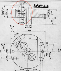
To solve for something more realistic, I took a look at the engineering drawings for the Curta Type II. In one of the drawings, there is a feature that is basically a cylindrical hole with a bottleneck added to it. This sketch represents the profile of the cut for that feature.
	sketch := dlineate.NewSketch()

	// Add elements
	start := sketch.AddPoint(6, 0)
	line1 := sketch.AddLine(6, 0, 9.4, 0)
	line2 := sketch.AddLine(9.4, 0, 9.4, -1)
	line3 := sketch.AddLine(9.4, -1, 8.1, -2)
	arc1 := sketch.AddArc(8.5, -2.4, 8.1, -2, 8.1, -2.7)
	line4 := sketch.AddLine(8.1, -2.7, 9.4, -3.8)
	line5 := sketch.AddLine(9.4, -3.8, 9.4, -8)
	line6 := sketch.AddLine(9.4, -8, 6, -8)
	line7 := sketch.AddLine(6, -8, 6, 0)
	arc2 := sketch.AddArc(6, 0, 6, 3, 8.1, -2.1)
	arc3 := sketch.AddArc(6, -5, 6, -8.3, 8, -2.5)

	// Add constraints
	// Constrain offset line to position the rest
	sketch.AddCoincidentConstraint(sketch.XAxis, start)
	sketch.AddDistanceConstraint(sketch.Origin, start, 6)

	// line points are coincident
	sketch.AddCoincidentConstraint(start, line1.Start())
	sketch.AddCoincidentConstraint(line1.End(), line2.Start())
	sketch.AddCoincidentConstraint(line2.End(), line3.Start())
	sketch.AddCoincidentConstraint(line3.End(), arc1.Start())
	sketch.AddCoincidentConstraint(arc1.End(), line4.Start())
	sketch.AddCoincidentConstraint(line4.End(), line5.Start())
	sketch.AddCoincidentConstraint(line5.End(), line6.Start())
	sketch.AddCoincidentConstraint(line6.End(), line7.Start())
	sketch.AddCoincidentConstraint(line7.End(), line1.Start())

	// line1 constraints
	sketch.AddParallelConstraint(sketch.XAxis, line1)
	sketch.AddDistanceConstraint(line1, nil, 3.4)

	// line2 constraints
	sketch.AddParallelConstraint(sketch.YAxis, line2)
	sketch.AddAngleConstraint(line2, line3, 135, false)

	// line3 constraints
	sketch.AddAngleConstraint(line3, line4, 90, false)

	// arc1 constraints
	sketch.AddDistanceConstraint(arc1, nil, 0.5)
	sketch.AddDistanceConstraint(arc1.Center(), line7, 2.5)
	sketch.AddTangentConstraint(arc1, line3)
	sketch.AddTangentConstraint(arc1, line4)

	// line5 constraints
	sketch.AddParallelConstraint(sketch.YAxis, line5)

	// line6 constraints
	sketch.AddParallelConstraint(sketch.XAxis, line6)
	sketch.AddDistanceConstraint(line6, nil, 3.4)

	// line7 constraints
	sketch.AddParallelConstraint(sketch.YAxis, line7)
	sketch.AddDistanceConstraint(line7, nil, 8)

	// arc2 constraints
	sketch.AddCoincidentConstraint(arc2.Center(), line1.Start())
	sketch.AddCoincidentConstraint(arc2.Start(), line7)
	sketch.AddCoincidentConstraint(arc2.End(), line3)
	sketch.AddTangentConstraint(arc2, line3)
	sketch.AddDistanceConstraint(arc2, nil, 3)

	// arc3 constraints
	sketch.AddCoincidentConstraint(arc3.Center(), line7)
	sketch.AddCoincidentConstraint(arc3.End(), line7)
	sketch.AddCoincidentConstraint(arc3.Start(), line4)
	sketch.AddTangentConstraint(arc3, line4)
	sketch.AddDistanceConstraint(arc3, nil, 3)

	// Solve
	err := sketch.Solve()
The resulting graph and clusters look like this:
The final solution looks like this (gray lines represent the X and Y axes):


